In Economics as Malignant Make Believe I showed that the derivation of the supply curve in mainstream (neoclassical) economics is nonsense because production costs are nothing like they are assumed to be. This made me wonder, however, what would happen if you’d use a more realistic model of production costs – What would production and supply look like then? This isn’t that hard to model, so I built a simulation model on a free afternoon. In the following, I will first explain the model and after that I will discuss the results of running the model at different settings as well as some limitations and implications. The explanation of the model is rather technical, so if you don’t really care about that, I recommend to skip straight to the results section.
The Model
Contrary to standard economic models, this is a dynamic model or a simulation, meaning that it takes time into account. Firms or companies in the model can respond to market prices and adjust their production levels by investing in new production facilities (called “production lines” in the model), and conversely, the market price responds to total supply. At any time there can be at most 10 firms in the model.
Some parts of the model are influenced by random noise, but the extent of the influence of randomness is controlled by parameters (and is kept well below 3% in most simulations). The reason for adding randomness is that without randomness all firms in the model act exactly the same, which would be rather unrealistic. (I’ll say something more about this below.) Random numbers come from random.org.
Production Costs
Production costs consist of a number of components. Mainstream economists assume that there are “fixed costs” and “variable costs”. The first do not depend on the number of units produced – they represent the initial investment for opening the factory (or farm, or whatever). Variable costs are the costs per unit produced. Mainstream economists believe that variable costs rise with an increase in production, but that has already been shown to be nonsense in the 1950s – “variable costs” are more or less flat (and thus not really “variable”). “Fixed costs” aren’t as “fixed” as they are supposed to be either, however. So-called “fixed costs” are the costs for buildings, machinery, and so forth needed for a certain production capacity. If a producer runs at 100% capacity, it produces the maximum number of units that can be made with the buildings, machinery, and so forth available. There is no point in adding more labor or inputs/resources if you are at 100% capacity – more workers would just stand by and watch, and more inputs would be equally useless if the available machines cannot handle them. Typically, fixed costs are very high and aren’t earned back until a producers is well over 50% capacity, and because of that, the vast majority of firms run at capacities between 80% and 100%. This means that in many cases, a (significant) production expansion is possible only by investing in another production line, which also would have to run at at least half capacity (and probably more) immediately to be profitable.
The costs of a company, then, consist of the following components:
- Costs of labor and input per unit produced. These costs are flat. In the model they are represented with a parameter, and can thus be set at any level desired.
- Costs of starting a new production line (i.e. investments). This too is a parameter of the model. Such costs are generally very high and usually require a bank loan.
- Maintenance costs of existing production lines. (Another parameter.)
- Administrative costs including the costs of marketing, sales, and so forth. In the model it is assumed that these costs increase with the size of production, but that the relation is not linear. Rather, there are economies of scale with regards to administration – managing and administrating a large company is cheaper per unit produced than managing and administrating a small company.
- Interests: the costs of aforementioned loans for opening up new production lines. In the model it is assumed that a firm uses its available money first to open a new production line, and only borrows from the bank if it doesn’t have enough money. Interest levels are another parameter of the model.
Thus, total costs TC of a firm in a model period are:
in which LC stands for the costs of labor and inputs/resources, MC for maintenance costs, AC for administrative costs, Int for interests, and Inv for investments.
in which Prod is the total number of units produced, p1 is a parameter of the model representing the costs of labor and inputs/resources per unit, r1 is a random number between -4.5 and 4.5 (with steps of 1, so there are 10 possibilities), and pr1 is a parameter that controls the effect of randomness. Obviously, if pr1 is set to 0, then there is no randomness in this respect. In most simulations, p1 and pr1 were set such that random variations in production costs per unit are at most 2.25%.
in which PL is the number of production lines and p2 is a parameter of the model representing maintenance costs per production line.
in which Prod is the total number of units produced, p3 is a parameter to take (dis-) economies of scale into account, p4 is a parameter to vary the administrative costs per unit (after taking economies of scale into account), and r2 and pr2 are a random number and parameter to set the effect thereof similar to r1 and pr1 (see above). In different simulations p3 was set at different values ranging from 0.2 to 1, and pr2 was set at a level to make the effects of randomness very minor but not completely negligible (i.e. similar to pr1).
in which BbII is the balance (here meaning current assets minus liabilities) before payment of interests and investments, which is assumed to be the sum of money borrowed from the bank if it is below 0 (and money stored in a bank account otherwise), and p5 is the interest rate. This is not entirely realistic as firms tend to have loans while having a positive balance, but this is only a very minor deviation. BbII is the balance (the sum of money the firm has or has borrowed) at the end of the previous model period plus income (from sales) in the current model period minus ( LC + MC + AC ). And min(BbII;0) returns 0 if BbII is positive and BbII if BbII is negative.
in which NewPL represents the number of new production lines opened in that model period, which is either 0 or 1 (meaning that firms can invest in at most one new production line per model period), and p6 is a parameter representing the costs of a new production line.
Income
It is assumed that all firms sell all units they produce, and that the market price is determined by the total supply. That is, the market price is the price at which all supply is sold. This is what the market price curve looks like (with supply on the x-axis and market price on the y-axis):
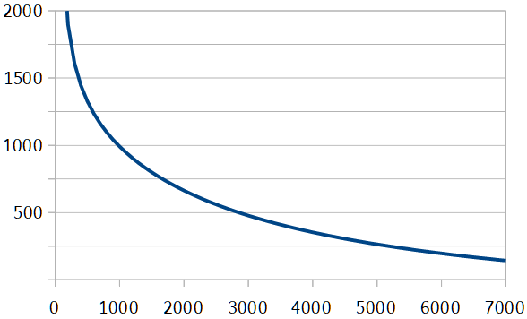 (Hence, this is a fairly traditional downwards sloping curve. It is, in fact, an idealization of the demand curve for ramen that was derived in Economics as Malignant Make Believe.)
The income of a firm is its total production multiplied with the market price.
Production, Investments, and Bankruptcy
At the end of each model period, all firms decide their production levels for the next period, whether to invest in a new production line or to close one of their existing production lines, and can go bankrupt.
A firm goes bankrupt if it has a negative balance (i.e. its liabilities are greater than its current assets) and a negative profit (meaning that it doesn’t have the money to pay interest to the bank). If a firm goes bankrupt, all its production lines disappear, and its production becomes zero. (Its debts also disappear.) A bankrupt firm cannot restart, but another firm can take its place in the model.
Decisions about changes in production level depend on the relation between average production costs and the market price.
in which AvgC is the average production costs per unit produced, TC is the total production costs for that time period, and Prod is the total number of units produced.
If AvgC is smaller than the market price, the firm increases the production of its existing production lines (if possible!). If it is larger or equal, it decreases production. (Note that this refers to production levels for the next model period.)
If a firm increases production, its new production target PTar is:
in which Prod is the production level in the current model period, PCap is the production capacity (i.e. the maximum the firm could produce with its current production facilities), price is the market price, and p7 is a parameter that sets the firm’s responsiveness to the market (in most simulations this was set at around 0.2).
If a firm decreases production, its new production target PTar is:
in which the only new variable, p8, is a parameter that sets the firm’s responsiveness to the market (in most simulations this was set at around 0.5). (It turned out that this parameter needed to be set a bit higher than p7 to allow the quick response to overproduction that is necessary to avoid bankruptcy.)
The actual new production level of existing production lines (not taking into account a new production line if there is one) in the next model period is further affected by randomness (simulating events outside the control of the firm’s management):
in which r3 and pr3 are a random number and a parameter to set the size of the random effect, respectively. (And the min function makes sure that production cannot exceed capacity.)
Production capacity PCap is simply the number of production lines multiplied with another parameter p9 that sets the capacity of individual production lines. (For sake of simplicity, it is assumed that all production lines are identical in their investment costs, maintenance costs, and capacity.)
A firm can open a new production line if the expected profit of a new production line exceeds a threshold set by another parameter. Whether it actually does so is affected by randomness, however. Yet another parameter sets the chance that a firm opens a new production line if it can do so. Obviously, if this is set at 100%, there is no effect of randomness. In most simulations this percentage was set at 60% or (a bit) higher.
Expected profit of a new production line is:
in which p10 is the production level of the new production line relative to the capacity of a production line p9 (p10 is usually set at around 65%, meaning that a new production line starts at 65% of capacity), p11 is the number of model periods over which the investment in the new production line is spread out (or in other words, the number of periods in which the investment must be earned back, which was usually set between 5 and 10), and all other variables were already specified above. Basically, what this does is calculate the difference between current total profit and the expected new total profit at current market price.
Conversely, a firm might close down an existing production line if it has more than 1 production line and if it would close one production line while keeping the same total production level (i.e. Prod) then production divided by maximum capacity (of the remaining production lines together) would drop below a level set by a parameter p13 (which in most simulations was set at around 85%). (Or in other words, even if with one production line less the utilization of remaining production capacity would be below this threshold.) As was the case with investing in a new production line, whether a firm actually closes a production line depends on chance. A parameter sets the chance that a firm closes a production line if it might do so (according to the preceding). This is, in fact, the same parameter that determines the chance of opening up a new production line. As mentioned, in most simulations this percentage was set at 60% or (a bit) higher.
A firm cannot close and open a production line in the same period (obviously).
Finally, there is one further parameter in the model that sets the production level (relative to capacity) of firms that have production lines at the beginning of a simulation. Any of the maximum 10 firms in the model can start with any number of production lines, but in most simulations they all start with 0 (i.e. they don’t exist yet). Any new firm (and any firm at the beginning of a simulation) starts without any money and without any debts.
Parameters and Random Numbers
The following table lists all parameters and random numbers used in the model. The rightmost column lists the base values for all parameters.
| p1 | Costs of labor and inputs per unit. | 100 |
| p2 | Maintenance costs per production line. | 10,000 |
| p3 | (Dis-) Economies of scale. (Administration costs.) | 0.5 |
| p4 | Administration costs. | 1,000 |
| p5 | Interest rate on bank loans. | 5% |
| p6 | Investment costs (for opening a new production line). | 100,000 |
| p7 | Market responsiveness (production increase). | 0.2 |
| p8 | Market responsiveness (production decrease). | 0.5 |
| p9 | Production capacity per production line. | 500 |
| p10 | Relative production level of new production line. | 65% |
| p11 | Return on investment period length. | 10 |
| p12 | Profitability threshold for investment. | 5,000 |
| p13 | Production level threshold for closing production line. | 85% |
| p14 | Production level at start of simulation. | 85% |
| r1 | Random number. Affects production. | |
| r2 | Random number. Affects administration costs. | |
| r3 | Random number. Affects new production level. | |
| r4 | Random number. Affects decision to open/close production line. | |
| pr1 | Sets effect of r1. | 0.5 |
| pr2 | Sets effect of r2. | 0.5 |
| pr3 | Sets effect of r3. | 0.5 |
| pr4 | Sets effect of r4. | 60% |
All random numbers are (derived from) integers between 0 and 9. In case of r1 to r3, 4.5 is subtracted. In case of r4, 1 is added and the result is divided by 10.
Any simulation is ran for at least 1000 steps (periods).
Running the Model (Results)
There are two ways to change the results of a simulation: replacing the random numbers, and changing one or more parameters. The first doesn’t lead to significantly different results, however. It changes which firms survive, which ones go bankrupt, which ones thrive, and so forth, but it doesn’t (substantially) change the number of firms that survive, total supply, “equilibrium” price, and similar outcomes, and those are the kind of results that matter.
As mentioned, the effect of randomness can be canceled (by setting pr1 to pr3 at 0 and pr4 at 100%), but this makes the behavior of all firms identical, meaning that they invest in new production lines or go bankrupt (etc.) together. Although other parameters co-determine what exactly happens, switching off randomness gives rather uninteresting (and unrealistic) results. Obviously, the other extreme – very high settings for the randomness-controlling parameters – results in very wild fluctuations. Because the point of the model is not to investigate the effects of randomness and randomness is merely added to the model to make firms non-identical, the best/most useful results are obtained by keeping the effect of randomness modest. This means that pr1 to pr3 are set such that the effects of randomness increase or decrease the variables they affect by 2.25% at most. Because the decision to open or close a production line is a major decision for a firm and many factors that aren’t part of the model affect such decisions, pr4 is best set at approximately 60% (meaning that there is a 60% chance that a firm opens or closes a production line if – according to the model – it has reason to do so).
If all parameters are set at their base levels (see table above), and there are no active firms in the market at the start of the simulation, then the simulation tends to stabilize for a while after 30 or 40 periods at 4 firms. There are small fluctuations in supply and price, but all four firms make a profit, and there is no room for a fifth. Market price more or less stabilizes at 159 on average (but fluctuates between 142 and 185), and average production costs are around 143. Eventually, one of the four will go bankrupt, however, and only three survive. One of the three will be significantly larger than the other two. If one firm has a small head start, then usually only 2 firms survive. (Market price around 157; average production costs around 138.) If one firm has a big head start, then none of its competitors survive. (Market price around 146; average production costs around 134.) In all cases, the market reaches a relatively stable “equilibrium” (despite fluctuations) at a level where no profitable investments in new production lines are possible.
We can change parameters one by one to see what happens. If the minimum profit threshold for investing in a new production line is lowered from 5000 to 500, meaning that firms even make investments if minimal profits are expected, then eventually only one firm survives. If, on the other hand, firms only invest when they expect a profit of at least 10,000 per period from the new production line, then more firms survive and all of them remain fairly small (2 or 3 production lines each; 6 firms in total). (Market price around 164; average production costs around 151.) Similarly, increasing the required time before return on investment decreases the number of surviving firms; decreasing the required time increases survival. Both “gambling” on small profits and a willingness to accept a very long time until an investment is earned back indicate a willingness to take risk, and consequently, both these findings suggest that low risk aversion pays off. A firm that is willing to take risks is – at least in this model – likely to end up with a monopoly.
If the size of production lines is doubled (from 500 to 1000) and their investment and maintenance costs as well, only 1 firm survives, but it tends to take a very long time until its last competitor goes bankrupt. If, on the other hand, the size and costs of production lines are halved, more firms (7 on average) survive. If only the investment costs are increased, the number of surviving firms also increases because none of them can take the risk of opening up another production line as soon as a (more or less) stable situation is reached. If investment costs are significantly decreased, only one firm survives.
If there are no economies of scale (i.e. p3 is set to 1 and pr3 and p4 are adjusted accordingly), then there is no advantage for large firms and more (small) firms survive (usually around 7). If there are diseconomies of scale (i.e. it is advantageous to be small), the number of surviving firms will be around 8. If size is an advantage, on the other hand, then less firms remain, but even at extreme settings of p3 often two firms survive.
Of the various parameters those with the biggest impact are the size of production lines and those that capture aspects of risk aversion. The bigger a production line (factory, farm, whatever) the less firms in the market can survive. The more willing firms are to take risk and to exploit even opportunities for small profits, the less firms survive.
If it is assumed that it is in the public advantage to have the lowest possible prices, then – unless there are no economies of scale whatsoever – it is in the public interests to have less firms. Monopolists produce at the lowest costs and sell at the lowest price. In this model they cannot set the price, but if they would set it higher than the market price, then competitors would emerge. Supply levels always “stabilize” at a level that corresponds to a market price that make it impossible for new competitors to emerge or for existing firms to significantly increase production.
Limitations and Implications (Discussion)
It must be emphasized that this is a “toy model” and not a serious contribution to economics. I made this model on a weekend afternoon partially because I was puzzled by questions raised by my earlier post Economics as Malignant Make Believe and partially to amuse myself. (Writing this post took much more time than building the model.) I cannot really judge how relevant the findings of this model are, so probably conclusions should be taken with a grain of salt. That said, this model is considerably more realistic than the overly simplistic and ill-founded standard model used to derive a supply curve by mainstream economists, and therefore, also more likely to be relevant for the real world.
Aside from it being a “toy model” there are obviously various limitations of the model. Most important is that firms do not have the ability to set prices. I thought about modeling that, but decided not to (for now at least) because it is far more complicated. Furthermore, the model does not take technological advances leading to productivity increases into account. Neither does it incorporate aging of production lines. And of course, it assumes that all production lines are identical in size and other relevant respects. And finally, aside from subtle differences due to randomness, all firms in the model are identical (and produce the exact same thing). All of these problems and limitations can be dealt with in a more complicated model, but I doubt that it will lead to different conclusions, which implies that it is most likely not worth the (considerable) effort.
Probably the most important of these limitations is that of price-setting versus price-taking, but that is also one of the hardest to model and at the same time the most predictable in its results. If firms would be able to set their own prices, then the production of the firm with the lowest price would be sold first, that of the second cheapest next, and so forth, until only firms are left that set their prices above the market price associated with the supply level of everything sold thus far plus the production of the next firm. This would drive prices down and would give an obvious advantage to the firm(s) with the lowest production costs. Thus, if there are any economies of scale – and usually that is the case – then size is an advantage, and by implication, the biggest firm would out-compete all of its competitors and establish a monopoly. Hence, while such a model would be considerably more complicated to build, it would probably lead to very similar (or even identical) conclusions as the model presented here.
A first conclusion of the model is that if there is a (downward sloping) curve that relates price to supply (and thus determines the market price at which all supply will be sold), then the actual price will more or less stabilize (with significant fluctuations) on a level just above average production costs, but not so far above it that new market entries or investments in new factories (etc.) are profitable. Hence, like the mainstream economic supply-and-demand model, this model can produce an “equilibrium” price – although it is a far less stable and fixed equilibrium and seems more like an “attractor” than a real “equilibrium” – but without offering a supply curve. (Nevertheless, it might be possible to derive a supply curve by keeping the market price fixed and then varying this fixed market price simulating the evolution of different stable production levels, but any point on such a “supply curve” would depend as much on the setting of the various parameters as on the market price.)
Secondly, willingness to take risk pays off. The more willing a firm is to exploit even small opportunities, the more likely it will get to dominate the market and even become a monopolist. This reminds me of the second half of Hegel’s famous Master / Slave Dialectic in which he argues that in a hypothetical confrontation between two individuals, the one willing to take risk (even to risk his life) will end up as master, while the more risk-averse individual will end up as his slave. Here, the firm willing to take risk (even to risk bankruptcy) will end up as monopolist, and the more risk-averse firm(s) will go belly up. (On the other hand, it might be the case that risk doesn’t help the monopolist directly, but kills off all its competitors. In that case, the monopolist is just the lucky survivor. It would then be an advantage if other firms are risk-takers. The current model cannot clarify which is an advantage – being a risk-taker oneself or competing with risk-takers (or both) – as it doesn’t allow different firms to have different setting with regards to risk aversion.)
A third conclusion is that – contrary to mainstream economic orthodoxy – monopolies are not necessarily a bad thing. If there are economies of scale, even if they are small, monopolists can produce and sell at the lowest cost. However, if there are significant barriers to market entry for new firms, then monopolies can abuse market power (but note that there is no such possibility in the model itself). For that reason, in markets where there are such barriers (such as “natural monopolies”) democratic control (or oversight, at least) is necessary to avoid such abuse. If there are no significant entry barriers, on the other hand, a monopolist has no real market power and new firms will enter the market if the monopolist sells too far above the market price. Consequently, welfare considerations suggest that monopolies in markets with high entry barriers (but only in such markets) should be nationalized and brought under democratic control, but even in such markets there should be no formal (i.e. legal, etc.) entry barriers because technological change may reduce (financial) entry barriers and enable new competitors to enter the market (which would force the former monopolist to decrease its production costs).
Fourthly, the model does not support the doctrine of the efficiency of free markets (another core dogma of mainstream economics). The model assumes a free market and under that condition a (more or less) equilibrium price and supply are reached, but those levels are such that existing firms and potential new entrants are deterred from making (further) investments – they are not the optimum levels from a welfare maximization point of view, but are well above those. (Optimum levels would be such that market prices would equal average production costs.) Furthermore, there is no reason why the equilibrium in the model could not be reached under other conditions. A monopolist could by means of step-wise production increases reach the same price and supply levels or even the optimum levels. It is true, of course, that the free-market condition creates an incentive for firms to act in such a way that the equilibrium is reached (while a monopolist does not automatically have such an incentive), but that only shows that such incentives are necessary, and not that a free market is the only way to create such incentives. Another possible objection to this conclusion is that the model doesn’t take price-setting and productivity increases leading to lower production costs into account. However, while this is true, it doesn’t change this conclusion – again, it only shows that incentives are necessary to make firms (or a monopolist) invest in research and development and in new technologies to increase productivity and lower their (or its) prices, but it does not imply that the free market is the only way to create such incentives. There may be more efficient ways to implement such incentives (democratic control, might work, for example), and they may even lead to optimal price and supply levels (rather than to levels that merely deter new investments in production).
A final remark about the limitations of this model (and thus its results) is in order. In Economics as Malignant Make Believe it was explained that a demand curve can have (almost) any shape, and because the price at which all supply is sold in this model is based on the demand curve, the market price curve could – at least in theory – have a very different shape as well. For example, it could look like the red line in the following graph (rather than the blue line):
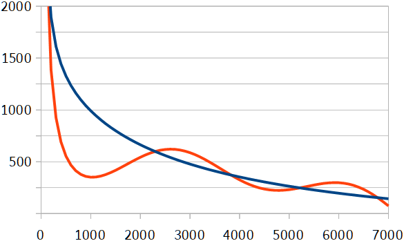 Perhaps unsurprisingly, if the red curve determines market prices, no stable situation emerges (or at least not with plausible settings of the various parameters). Supply and market prices fluctuate wildly, and there are firms going bankrupt and starting up all the time. And none of the aforementioned conclusions follow (except for the fourth, perhaps). Whether curves like the red line actually occur, I don’t know however, and as long as the curve is continuously downward sloping, the above conclusions do follow.
If you found this article and/or other articles in this blog useful or valuable, please consider making a small financial contribution to support this blog 𝐹=𝑚𝑎 and its author. You can find 𝐹=𝑚𝑎’s Patreon page here.