Climate scientists use supercomputers and extremely complicated models to predict the future climate, but there is a shortcut that can be used to predict average global warming. The key to that shortcut is the following simple formula:
$$ \Delta T_{anom.} = \frac {ECS \times ( C_{atm.} – 280 )} {280} \: – \: \psi,$$ in which \(\Delta T_{anom.}\) is the average temperature anomaly (or average global warming), \(ECS\) is “Equilibrium Climate Sensitivity”, \(C_{atm.}\) is atmospheric carbon (in ppm CO₂ equivalent), and \(\psi\) (from Greek ψῦχος, meaning “cold”) stands for various cooling effects. If you have the values of the variables on the right side of the equal sign, then the calculation is very easy. All that is missing (then) is an estimate of the uncertainty margin.
\(ECS\) — Equilibrium Climate Sensitivity
There is some disagreement about the best estimate of \(ECS\).1 Steve Sherwood and colleagues suggest that it is 3.1°C (with 66% uncertainty range: 2.6~3.9°C; 95%: 2.3~4.7°C).2 James Hansen and colleagues suggest that it is 4.8°C (with 95% uncertainty range: 3.6~6.0°C).3 So-called “cold models” are closer to the Sherwood estimate; so-called “hot models” are closer to the Hansen estimate.
The main argument in favor of Sherwood/cold models is that \(ECS=3.1°C\) results in global average temperature predictions that track actually measured warming very closely, but only if \(\psi\) is zero, or in other words, if there are no significant cooling effects. The main argument in favor of Hansen/hot models is that \(\psi\) is probably (or almost certainly) not zero, and thus, that \(ECS=3.1°C\) underestimates warming. However, \(ECS=4.8°C\) results in very high temperature estimates and whether \(\psi\) is large enough to explain the difference with actual measurements is presently unclear.
\(\psi\) — Cooling Effects
The main cooling effect mentioned by Hansen and colleagues is “aerosol cooling”, which is caused by certain kinds of pollutants in the atmosphere, such as soot, dust, PM2.5, sulfates, and much more. Some of these end up in the atmosphere due to natural processes, but much of it is of an industrial origin. A figure in the paper by Hansen and colleagues suggests that \(\psi_{aerosol{\text -}cooling}\) is roughly 1.3°C or 1.4°C, which would completely explain away the difference between predictions based on \(ECS=4.8°C\) and actual temperature measurements. However, this high estimate of \(\psi_{aerosol{\text -}cooling}\) (i.e., the aerosol cooling effect) is controversial.
A recent paper by Kyle Armour and colleagues suggests that sea-surface temperature patterns may have slowed down global warming, implying that this is (probably) another cooling effect on the short and mid term.4 Another cooling effect that may play a significant role on the longer term has to do with the Atlantic Meridional Overturning Circulation (AMOC). A “collapse” thereof would lead to approximately 0.5°C of global cooling and local cooling effects (in parts of Europe and North America) of 4 to 10°C. However, the extent of warming needed to trigger this collapse is quite high (namely, 4°C, with an uncertainty range of 1.4~8°C), so this is not something that needs to be taken into account in most calculations.
In any case, \(\psi\) is the sum of various specific effects, such as aerosol cooling, sea-surface temperature patterns, and so forth. It’s hard to say how high \(\psi\) should be for a plausible prediction and it must further be noted that some of the effects that are part of \(\psi\) are themselves dependent on what we do. This is most obvious in case of aerosol cooling – the less aerosols we emit (i.e., the less we pollute), the smaller this cooling effect will be. Personally, I think that anything higher than \(\psi=1.4°C\) and anything lower than \(\psi=0.4°C\) is extremely implausible, but that still results in quite a large range.
- low: \(ECS \approx 3.1°C\) and \(\psi \approx 0°C\);
- high: \(ECS \approx 4.8°C\) and \(\psi \approx 1.3°C\);
and these two may give very similar predictions at relatively low values for \(C_{atm.}\) (that is, values close to those what we have now), but will start to deviate significantly at higher levels of atmospheric carbon.
\(C_{atm.}\) — Atmospheric Carbon
The current value for atmospheric carbon in ppm (parts per million) CO₂-equivalent can be found at http://www.co2.earth/. (It is 427 at the time of writing.) To calculate the level of atmospheric carbon for which you want to make an estimate of the warming effects you need to know emissions between now and then, as well as how much of those emissions end up in the atmosphere.
$$ C_{atm.} = C_{atm.{\text -}now} + \frac {(1 – seq) \times \sum E_C} {7.76},$$ in which \(C_{atm.}\) is the level of atmospheric carbon you want to use in the first equation above, \(C_{atm.{\text -}now}\) is the starting level (for example, the level at the beginning of the current year), \(seq\) is the percentage of carbon emissions that are “sequestered”, meaning that they end up in the oceans or elsewhere and thus not in the atmosphere, and \(\Sigma E_C\) is the sum of yearly carbon emissions in gigatons CO₂-equivalent between now and the time of \(C_{atm.}\).
\(1 – seq\) is the percentage of carbon emissions that end up in the atmosphere. Estimates of \(1 – seq\) are typically in the 45~50% range, but it must be taken into account that there are reasons to believe that carbon sequestering might work less well at higher average temperatures, and thus, that this percentage might be a (little bit) higher in case of some scenarios. (Furthermore, there are some uncertainty margins involved here, but those are also taken into account in the simplified uncertainty margins suggested below.)
This leaves estimating \(\Sigma E_C\), which is probably the hardest part of making a prediction of average global warming. To calculate \(\Sigma E_C\), you need a spreadsheet with yearly carbon emissions (in gigatons CO₂-equivalent) and add those up. Current yearly emissions (i.e., \(E_C\) for this and previous years) are about 50 Gt, but you may want to look up more exact numbers. Then, based on some scenario that you think is plausible, you decide the likely values for \(E_C\) in subsequent years up to and including the year for which you want to calculate \(C_{atm.}\). To see whether your scenario looks OK, it is easiest to make a graph (with the inbuilt graph utility of the spreadsheet program you are using). There are some important things to take into account, however. Most important among those is “residual emissions”.
Residual emissions are carbon emissions that are effectively unavoidable at the current state of technological development and other relevant circumstances. Estimates of residual emissions differ, but my calculations (based on researching the residual emissions for various industries, agriculture, transport, and so forth and multiplying those with the relative emission contributions of those various sectors) suggests that about 37% of current carbon emissions are residual. Technological development will reduce that percentage, but slowly, and especially residual emissions for the agricultural sector are not likely to decrease much. (Or at least not with a very significant decrease in human population size.)
Secondly, technology to capture and store carbon directly from the atmosphere exists, but requires so much energy that it can never play a significant role in atmospheric carbon reduction.
Thirdly, there are important feedback effects between economic growth and several other relevant variables. Economic growth is closely associated with an increase in energy use. Higher levels of warming are likely to seriously depress economic growth for a number of reasons, and lower economic growth is likely to slow down technological development and investment in “green” technology.5
Fourthly, an even more important feedback effect is that high levels of average global warming will lead to so much havoc that this will – in one way or other – reduce further emissions. At 2.5°C or 3°C average global warming (and possibly even at 2°C), disruption of trade networks, widespread droughts and famines, refugees in the millions, cascading societal collapse, ever-increasing “natural” disasters and a long list of other problems make it impossible for manufacturing industry and other economic sectors to continue operating “as usual”, for example. It is largely for this reason that runaway global warming is very unlikely – human civilization would be destroyed completely before we could emit the amount of CO₂ needed for that.6
Much more can be said about what is more and less likely with regards to scenarios of future carbon emissions, but if you come up with a scenario that looks plausible to you, there is a good chance that you actually have a more realistic scenario than those the IPCC is using, as those tend to ignore all three of the above “important things to take into account”.
Uncertainty Margins
Most models and estimates of climate sensitivity tend to have fairly similar uncertainty margins, and consequently, the easiest way to calculate the uncertainty margins for your estimate of average global warming is to use an approximation thereof.
- The 66% uncertainty range is from (\(0.83 \times \Delta T_{anom.}\)) to (\(1.25 \times \Delta T_{anom.}\)).
- The 95% uncertainty range is from (\(0.66 \times \Delta T_{anom.}\)) to (\(1.65 \times \Delta T_{anom.}\)).
That’s all.
An Example
As an example, consider the following yearly carbon emission curve:
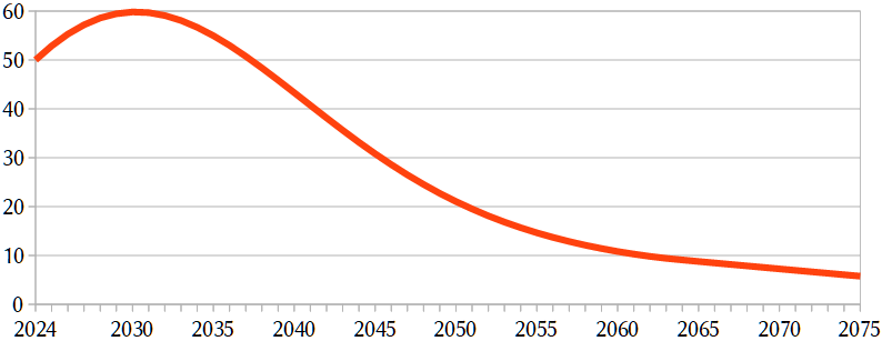 It starts at 50 Gt, which is roughly what has been emitted recently. Average yearly emissions are still increasing, which is unlikely to stop in the near future, especially considering all the new fossil-fuel-related infrastructure being built and planned. Nevertheless, in this scenario, carbon emissions start dropping quite rapidly from the early 2030s onward. It is assumed here that rich industrialized nations make some genuine effort to reach their official goals of carbon-neutrality by 2050, but also that they will not quite reach this due to the problems of residual emissions and opposition to climate policies. China and India aim for carbon-neutrality by 2060 and 2070, respectively, which is a further reason why the line continues to slope downwards. The line never reaches zero, however, because of aforementioned residual emissions and the implausibility of large-scale carbon capture from the atmosphere. I’d say that this is about the most optimistic scenario that avoids ascending to cloud-cuckoo land, although it’s getting nearly there. I’m not sure whether we can actually reach such a drastic reduction of carbon emissions without completely abolishing modern agriculture and most industry, but let’s be optimistic (or insane?) and ignore that.
The target year is 2075. That is, we want to know average global warming or \(\Delta T_{anom.}\) for that year. It should be noticed that this warming level may not be reached in 2075 itself in this scenario, as there is some time lag involved (but it is controversial how long that time lag is – estimates are typically a couple of years to a decade or so for the most important temperature effects). To calculate \(\Delta T_{anom.}\) for 2075, the first thing we need to know is \(\Sigma E_C\) for the period 2024–2075. That is just the sum of the yearly values shown in the figure above, which is 1489 Gt.
$$ C_{atm.} = C_{atm.{\text -}now} + \frac {(1 – seq) \times 1489} {7.76}.$$ \(C_{atm.{\text -}now}\) is the average atmospheric carbon level at the beginning of the period, which is about 425 ppm (rounding down a bit). Usually, I use \(1 – seq=0.45\) (meaning that 45% of emissions end up in the atmosphere), which is a rather conservative estimate. Considering that 1489 Gt of CO₂-e is quite a lot, it is probably more plausible that the percentage should be a bit higher, but let’s be cautious and use 48%. Then,
$$ C_{atm.} = 425 + \frac {0.48 \times 1489} {7.76} = 517 ppm,$$ which can then be substituted for \(C_{atm.}\) in the first equation:
$$ \Delta T_{anom.} = \frac {ECS \times ( 517 – 280 )} {280} \: – \: \psi.$$ For \(ECS\) and \(\psi\) two variants were suggested above. In case of the low variant we get:
$$ \Delta T_{anom.} = \frac {3.1 \times ( 517 – 280 )} {280} = 2.6°C.$$ In case of the high variant:
$$ \Delta T_{anom.} = \frac {4.8 \times ( 517 – 280 )} {280} \: – \: 1.3 = 2.8°C.$$ These are so close together, that I’d just pick the average of the two variants, that is, 2.7°C of average global warming. The 66% uncertainty range is (\(0.83 \times 2.7°C = 2.2°C\)) ~ (\(1.25 \times 2.7°C = 3.8°C\)) and the 95% uncertainty range is (\(0.66 \times 2.7°C = 1.8°C\)) ~ (\(1.65 \times 2.7°C = 4.5°C\)).
In short, the example scenario suggests 2.7°C of average global warming with a 2.2~3.8°C 66% probability range and a 1.8~4.5°C 95% probability range. How (im-)plausible is that? Well, according to a very recent survey by the Guardian, 77% of IPCC-affiliated climate scientists surveyed expect 2.5°C or more average global warming. So, if anything, this example may be on the optimistic side (but I already said so above — twice).
Effects
But what does that number mean? What are the effects of 2.7°C of average global warming? (Remember that this number is just the result of one example scenario, and that scenario may be wrong for all kinds of reasons – again, it is an example.) Climate models don’t just give a single average global warming value, but instead model temperatures, precipitation, and various other climate variables. Average global warming (in the model) is just a derivative of those more detailed predictions. The other way around, there is a large body of research on the effects of various levels of warming on various spatial scales. Fortunately, Mark Lynas summarized much of that research in his book Our Final Warning (2020),7 which systematically describes the effects of increasing levels of warming with six chapters for 1°C to 6°C. So, if you want more than just a number, I recommend reading that.
If you found this article and/or other articles in this blog useful or valuable, please consider making a small financial contribution to support this blog, 𝐹=𝑚𝑎, and its author. You can find 𝐹=𝑚𝑎’s Patreon page here.
Notes
- See this post.
- Steve Sherwood et al. (2020), “An assessment of Earth’s climate sensitivity using multiple lines of evidence”, Review of Geophysics 58.4: e2019RG000678.
- James Hansen et al. (2023), “Global Warming in the Pipeline”, Oxford Open Climate Change 3.1: kgad008.
- Kyle Armour et al. (2024), “Sea-surface temperature pattern effects have slowed global warming and biased warming-based constraints on climate sensitivity”, PNAS 121.12: e2312093121.
- I have written about some of these issues as well as the previous point most recently in Capitalism and Climate Collapse.
- The Stages of the Anthropocene – Revisited series was trying to model this, but aside from the last episode, I haven’t re-uploaded this series yet.
- Mark Lynas (2020), Our Final Warning: Six Degrees of Climate Emergency (London: 4th Estate).